One statistical description measured during a random shake test is the Control Spectrum. Specifically, this variable is often the output of an accelerometer mounted to the shaker table. The sensor’s voltage output is scaled to engineering units of acceleration, typically gravitational units (g’s) sampled at a fixed interval, Δt. This time-sampled history is transformed to the frequency domain using the Fast Fourier Transform (FFT). In this process, a series of “snapshots” from the continuous time waveform are taken and dealt with sequentially.

Each snapshot is multiplied by another sampled time history of the same length, called a window function. The multiplied window function serves to smoothly taper the beginning and end of each time record to zero, so that the product appears to be a snapshot from a signal that is exactly periodic in the N Δt samples observed. This is necessary to preclude a spectrum-distorting convolution error that the FFT would otherwise make. The resulting discrete complex spectrum has nominal resolution of Δf = 1/NΔt and g amplitude units. However, every spectral amplitude computed is actually greater than what would result from detecting the amplitudes of a bank of perfect “brickwall” analog filters of resolution Δf.

Each complex spectrum is prepared for averaging by multiplying each complex amplitude by its own conjugate. This results in a real-valued “power” spectrum with g² amplitude units. To correct the over-estimated amplitude, each squared magnitude is divided by the equivalent noise bandwidth, kΔf (Hz) of the filters synthesized by the FFT. The value of the constant, k, is determined by the shape of the window function. The most common of these is called a Hann window (sometimes Von Hann or Hanning) for which k equals 1.5. The resulting amplitude units are now g²/Hz and the spectrum is said to have Power Spectral Density scaling.

The final step in the process is to ensemble average the current spectrum with all of those that have preceded it. The resulting average is called a Power Spectral Density (PSD) and it has the (acceleration) units of g²/Hz. The averaging is done using a moving or exponential averaging process that allows the averaged spectrum to reflect any changes that occur as the test precedes, but always involves the most recent DNΔt/2 seconds of the signal. D is the specified number of degrees-of-freedom (DOF) in the average, numerically equal to twice the number of (non-overlapping) snapshots processed.

If the snapshots are taken frequently enough not to miss any time data, the process is said to be operating in real time (as it must to control the signal’s content). If the process runs faster, the snapshots can actually partially overlap one-another in content. When the successive windows overlap, the resulting complex spectra contain redundant information. The degrees-of-freedom setting is intended to specify the amount of unique (statistically independent) information contained in the averaged Control spectrum. When overlap processing is allowed, the number of spectra averaged must be increased by a factor of [100/(100-% overlap)] to compensate for this redundancy.

The resulting PSD describes the frequency content of the signal. It also echoes the mean and the variance. The (rarely displayed) DC value of the PSD is the square of the mean. For a controlled acceleration (or velocity) shake, this must always be zero – the device under test cannot depart from the shaker during a successful test! Since the mean is zero, the RMS value is exactly equal to the standard deviation, σ. The area under the PSD curve is the signal’s variance (its “power”), σ². The term power became attached to such “squared spectra” when the calculation was first applied to electrical voltages or currents. (Recall that the power dissipated by a resistor can be evaluated as i²R or E²/R.)

It bears mentioning that long before real-time control of a random vibration signal was possible, random vibration test were conducted using a “white- noise” generator and a manually adjusted equalizer to shape the spectrum. Filter-based signal analysis was employed with a human “in the loop” to achieve some semblance of spectral control. In that same era, the PSD was formally defined by the classic Wiener-Khintchine relationship as the (not so fast!) Fourier transform of an Autocorrelation function. An autocorrelation is defined by the equation:

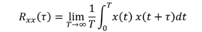
In essence, the autocorrelation averages the time history multiplied by a time-delayed image of itself. The symmetric function of time that results was often used to detect periodic components buried in a noisy background. The “squaring” of an autocorrelation would reproduce the periodic signal with greater amplitude, rising above the random noise background. In the process, it echoed the signal’s mean and variance. When you auto-correlate x(t), the R_xx(τ) amplitude at lag time τ= 0 is equal to σ² + μ². As the lag time approaches either plus or minus infinity, the correlation amplitude collapses to μ². Thus if the signal is purely random, the autocorrelation amplitude varies smoothly between the mean-square and the square of the mean.

CI Blog