
If you don’t excite a structure at its natural frequency, then how can you know what it is? This is an important item to discuss.

Well, this is an area where I find people often get confused. Many times I hear people say that they have to tweak and tune the excitation frequency so that they get the excitation right at the natural frequency otherwise the frequency will not be identified properly. I also hear people say that the excitation method must have broadband energy at all frequencies otherwise the system will not be excited properly.
There is a misconception that the frequency of excitation must be exactly at the natural frequency otherwise the results are not valid. Well this is not really a problem with the way we do frequency response testing and how we extract parameters from measured data to estimate the frequency and damping for a system.
So let’s discuss some of this and help you to understand why we really don’t need to excite a structure exactly at its natural frequency when we run a test -but we do have to make sure that the data we collect is good data because there is no substitute for good data.
Now let’s take a step back to something a little simpler and more commonly understood. Let’s look at a very simple straight line fit of some measured data. We are going to perform a least squares error minimization for the data presented in Figure 1. Now we know we can fit any line to the data but for this set of data it seems that a first order fit makes the most sense. Of course the model we are going to use is
y = mx + b
and there are two parameters that define the line, namely the slope and y intercept.
The data and fit of the data is shown in Figure 1. Now let’s look very closely at the data. We know that we can compute the slope, but did we ever really measure the slope? Not really –we measured data and then fit a mathematical function to that data which is then used to obtain the slope –but technically speaking we did not measure the slope. And let’s also look at the y intercept. If you look closely you will see that we never measured data that directly obtained the y-intercept. But certainly we would say that we could obtain the y-intercept but we really never actually measured it, did we? And let’s take this just one step further to see if we could obtain the value of the y function for a given value of x, let’s say 0.707. But we never actually measured the function for that particular value of x –but we would say that we know what it would be from the function we fit. I think we are all comfortable we these statements and the values that we obtain –right?

Figure 1: Example of Simple Straight Line Fit
So now let’s apply this logic to the mathematical function that is used to represent a single degree of freedom frequency response function. We can write the system transfer function in partial fraction formfor a single degree of freedom system as
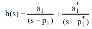
and we can also write the frequency response equation as

First we need to realize that this function is written as a function of frequency and it contains two constants which are the pole, p, and the residue, r; these are the two parameters that we need to extract (just like we did for the slope and y-intercept for the straight line). Now we can evaluate this function at a series of frequencies spaced delta f apart. This is shown in Figure 2. These data points are the set of data we collect when a frequency response measurement is made. We can fit a line to the data where the line is the complex frequency response function and extract the parameters of interest.
I can make the same argument that was made for the straight line here for the frequency response function. We are going to fit a line to the measured data and extract several key parameters that define that line. These are namely, the pole and the residue. And just like we argued for the straight line I do not necessarily need a data point exactly at the natural frequency to obtain an estimate of the pole or residue. As long as I have good data that represents the function, I can fit this simple single degree of freedom model to the measured data to extract the parameters of interest which are the poles and residues.

Figure 2 – Conceptual SDOF Curvefit
Now of course I can extend this from a single degree of freedom system to a multiple degree of freedom system and the problem just gets mathematically more complicated –but it is the same process overall. A multiple degree of freedom frequency response measurement is shown in Figure 3.

Figure 3–Conceptual MDOF Curvefit
Data is obtained at selected frequency spacing and there is no need to make sure that the frequency data points coincide exactly with the precise natural frequencies for the modes obtained from the parameter estimation process. But surely I have to remind everyone that the data that is collected must be obtained using the best of measurement methodologies to assure that there is little variance between the data collected and the line that is used to describe the data and for the extraction of the poles and residues.
So I hope that this little explanation helps to clarify the fact that the measured data does not necessarily need to lie exactly on the precise natural frequency for the system. The process of modal parameter estimation (which is really nothing more than a very elaborate least squares error minimization process) where parameters, namely the poles and residues, are extracted. If you have any other questions about modal analysis, just ask me.
Join Dr. Peter Avitabile for an upcoming webinar.