Dynamic Signal Analysis Basics
DSA is often referred to Dynamic Signal Analysis or Dynamic Signal Analyzer depending on the context. DSA uses various technologies for digital signal processing. Among them, the most fundamental and popular technology is based on the so-called Fast Fourier Transform (FFT). The FFT transforms the time domain signals into the frequency domain. To perform FFT-based measurements, it is important to understand the fundamental issues and computations involved.
Crystal Instrument’s analyzers fully utilize the FFT frequency analysis methods and various real time digital filters to analyze the measurement signals. The Fourier Transform is a transform used to convert quantities from the time domain to the frequency domain and vice versa. In the classical sense, a Fourier transform takes the form of

For discrete sampled signals, this can be expressed as

Where:
x(n): samples of time waveform
n: running sample index
N: total number of samples or “block size”
k: finite analysis frequency, corresponding to “FFT bin centers”
X(k): discrete Fourier transform of x(k)
The most important parameter to consider before performing an FFT is the sampling rate. The Nyquist-Shannon sampling theorem states that if a system uniformly samples an analog signal at a rate that exceeds the signal’s highest frequency component by a factor of at least 2 then the original analog signal can be recovered exactly from the discrete samples.

However, in many cases, the bandwidth of a given signal remains elusive and consequently the Nyquist frequency is unknown. To address this challenge, all of Crystal Instruments’ DAQs are equipped with anti-aliasing filters. This filter serves to limit the upper threshold of the signal frequency, effectively preventing aliasing.

Ideally, the cutoff frequency should be exactly half the sampling rate according to the Nyquist-Shannon sampling theorem. However, this would require a ‘brick wall’ filter, where all frequency components equal to or less than the Nyquist frequency are passed through without any attenuation and where all frequency components above the Nyquist frequency are completely attenuated. A real anti-aliasing filter will have a frequency response like the plot depicted below.
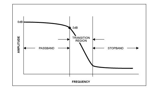
Crystal Instruments incorporates anti-aliasing filters with a transition region initiating at 0.45 times the sampling rate, and the cut-off frequency is adjusted accordingly.

With this cut-off frequency, we are assured that the acquired data is uncontaminated by aliased signals. By integrating the anti-aliasing filter alongside an appropriately chosen sampling rate, it becomes possible to conduct accurate spectral analysis.
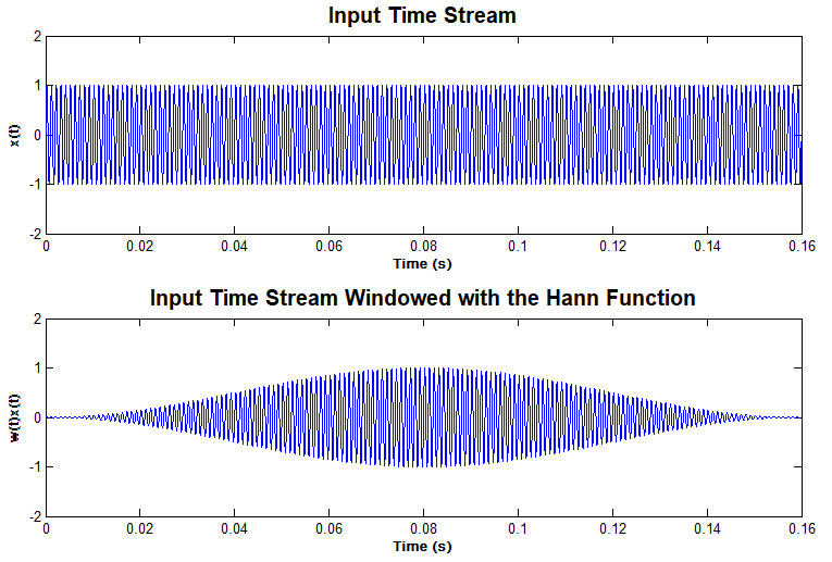
A caveat of the Fourier Transform is that it assumes a time signal is periodic and infinite in duration. When only a portion of a signal is analyzed, the block must be truncated by a data window to preserve frequency characteristics. To reduce the edge effects, which cause leakage, a window is often given a shape or weighting function. For example, a window can be defined as:
w (t) = g(t) -T/2 < t < T/2
= 0 elsewhere
where g(t) is the window weighting function and T is the window duration.
The data analyzed, x(t)’ are then given by:
x(t) = w(t)x(t)’
where x(t)’ is the original data and x(t) is the data used for spectral analysis.
Since windowing attenuates a portion of the original data, a certain amount of correction must be made to get an un-biased estimation of the spectra. In linear spectral analysis, an Amplitude Correction is applied; in power spectral measurements, an Energy Correction is applied.
The linear spectrum is useful for analyzing periodic signals. You can extract the harmonic amplitudes by reading the amplitude values at those harmonic frequencies. Most DSA products use the following steps to compute a linear spectrum:
Step 1
First a window is applied:
x(t) = w(t)x(t)’
where x(t)’ is the original data and x(t) is the data used for the Fourier transform.
Step 2
The FFT is applied to x(t) to compute X(k).

Step 3
Averaging is applied to X(k). Here the averaging can be either an Exponential Average or Stable Average. Result is Sx'.
S'x = Average(X(k))
Step 4
To get a single-sided spectrum, double the value for symmetry about DC and apply the AmpCorr factor.
Sx = 2S'x ∙ AmpCorr
where AmpCorr is the amplitude correction factor, defined as:
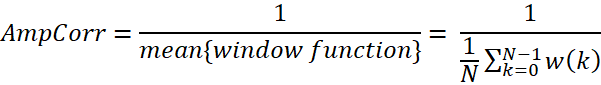
where w(k) is the window weighting function.
This correction will make the peak or RMS reading of a sine wave at specific frequency correct regardless of the chosen data window. For example, if a 1.0-volt amplitude 1 kHz sine wave sampled at 6.4 kHz is truncated with a Hann window and analyzed with a linear spectrum, the following APS will be generated:

In power spectrum measurements, window amplitude correction is used to get un-biased final spectrum amplitude reading at specific frequency. In PSD or energy spectral density (ESD) measurements, window energy correction is always used to get an un-biased spectral density or energy reading. Similar to the amplitude correction, the energy correction is a scalar value defined as:

where N is the number of samples and w(k) is the window function.
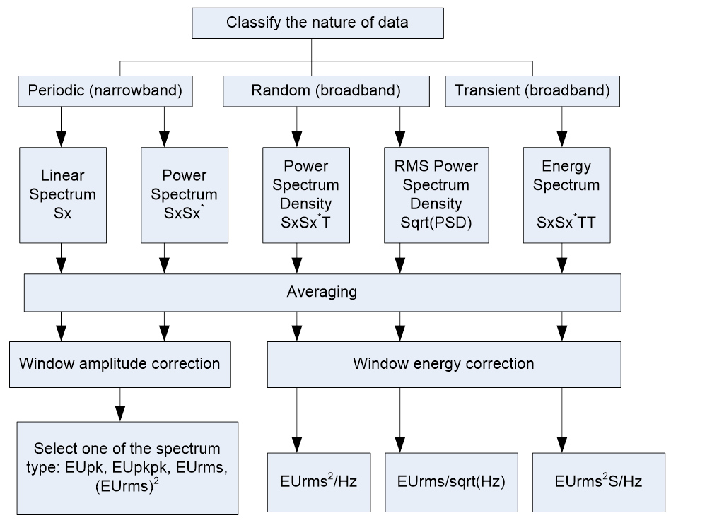
Making an appropriate spectrum selection is crucial for acquiring meaningful data. Depending on the scenario, an APS may provide valuable insights, while in other instances, examining the power or energy spectrum may be more suitable. The choice of spectrum should align with the nature of the signal under analysis, which can be categorized into three types.
1. Periodic Signals - These can be the signals measured from a rotating machine, bearing, gearing, or anything that repeats. In this case we would be interested in amplitude changes at fundamental frequencies, harmonics, or sub-harmonics. In this case, you can choose a spectrum type of EUpk, EUpkpk or EUrms.

2. Random Signals - It does not have obvious periodicity therefore the frequency analysis could not determine the “amplitude” at certain frequencies. However, it is possible to measure the rms. level, or power level, or power density level over certain frequency bands for such random signals. In this case, you must select one of the spectrum types of EU2rms/Hz, or EUrms/√Hz, which is called power spectral density, or root-mean squared density.
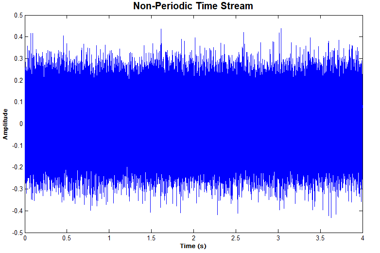
3. Transient Signals - It is neither periodic, nor stably random. In this case, must select a spectrum type as EU2/Hz2, which is called energy spectrum.

In many applications, the nature of the data cannot be easily classified. Care must be taken to interpret the data when different spectrum types are used. The flow chart below provides a general guideline for spectrum and measurement selection.