
Digital Filters & Resampling in Post Analyzer
Introduction | Download Paper
Digital filters are powerful tools utilized during the data conditioning phase to analyze signals. These filters empower users to augment signal processing capabilities by integrating them with other data conditioning modules, thus generating advanced post-analysis functionalities. Among the primary types of real-time digital filters are the Decimation filter, the FIR (Finite Impulse Response) filter, and the IIR (Infinite Impulse Response) filter.
Digital filters serve as powerful instruments for real-time signal filtering, facilitating the application of FFT (Fast Fourier Transform) and time-based analysis via the Post Analyzer platform. Users have the capability to finely adjust filter characteristics to suit exact requirements, leveraging a graphical design tool for filter modeling. This tool simplifies the visualization of filter performance, with the vertical axis corresponding to decibels (dB) and the horizontal axis corresponding to relative frequency.
An example use case involves analyzing the energy distribution over time within a specific frequency band, rather than across the entire spectrum. This is achievable by designing a band-pass filter, followed by the application of an RMS (Root Mean Square) estimator to the filtered output, offering insights into signal dynamics within the selected frequency range.
The Post Analyzer software, which will be explored in greater detail subsequently, supports these processes by allowing users to define real-time filters and analyze signals effectively. The content of this paper is taken from the Post Analyzer user manual.
Digital Filters
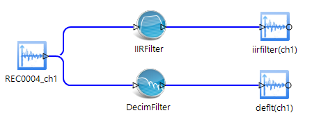
There are two approaches to signal processing illustrated in the provided figure. The first involves processing the native measured signal (CH1) through an IIR Filter to generate a filtered signal (iirfilter(ch1)), which is then analyzed by an RMS estimator to produce the signal rms(iirfilter(ch1)). The alternative method connects CH1 to a Filter_RMS module that combines filtering and RMS estimation into one process, resulting in a signal named filter_rms(ch1).

To utilize digital filters or other data conditioning operators, users should first select the "Data Conditioning" button located at the top of the screen. This action will prompt the opening of the Data Conditioning module. Within this module, users can then select and drag the desired operator from the bottom of the screen onto the data conditioning map displayed above the operators. Subsequently, users can establish connections by clicking and dragging a line from the input source to the chosen operator. Upon completion, the output will be automatically generated and named based on the selected operator. Each circle on the left side of the operator symbolizes an input requirement, while those on the right represent outputs. An example of this process is illustrated in the figure below.

One example of digital filter implementation would be if a user wants to look at the RMS value over time within the 100 Hz to 200 Hz and 1000 Hz to 2000 Hz ranges separately. This can be done by deriving two output streams from the native channel 1, then applying the band-pass filter to each path as shown below.

In another example, the user might want to look at the very fast time characteristics of a channel at high frequency, and the same channel at a very low sampling rate. This can be done by applying a decimation filter to the native time stream as shown below. The native channel time stream is split into two streams so that the signal from the same channel is recorded at both high and lower sampling rates.
There are three primary types of real time digital filters: IIR, FIR, and decimation filters. For FIR and IIR filters in the PA software, users can specify low-pass, high-pass, band-pass or band-stop types, or fixed low-pass, fixed high-pass, fixed band-pass, fixed band-stop or all pass (no band filter) types with several different methods. This paper first explains the theory about filter design, and then introduces the operations within the Post Analyzer software and the Spider hardware.
The goal of filter design is to calculate a series of filter coefficients based on the user specified criteria. The criteria are often described by following variables:
Number of Filter Coefficients: this is also known as the order of the filter. The filter order defines the number of delay elements used in the filter. A lower order filter consists of a fewer number of coefficients. A low order filter responds relatively faster than a higher order filter; that is, there is less of a time lag in the output of the filter.
Decimation Filter: A decimation filter is used to improve the performance of digital filters, particularly when the cutoff frequency (fc) is very low compared to the sampling frequency (fs), which can lead to distortion or divergence in the filter's response. Our Post Analyzer software incorporates a decimation filter ahead of the band-pass filter. This approach ensures that digital filters can be effectively applied even when the ratio of fc to fs is exceptionally low. By combining decimation with filtering, it becomes possible to accurately analyze frequency content at very low frequencies, for instance, below 10Hz, with a sampling frequency of 48kHz. The software offers various settings, including the option to apply no decimation or to apply a decimation ratio of up to 1:32 before applying an FIR or IIR filter. The default setting is to have no decimation filter applied. The decimation filter itself consists of a low-pass filter followed by a decimator, which together enhance the filter's ability to process low-frequency signals.
Cutoff Frequencies: For low-pass and high-pass filters or fixed low pass and fixed high pass filters, only one cutoff frequency is needed. Band-pass and band-stop filters or fixed band-pass and fixed band-stop filters require two cutoff frequencies to fully define the filter shape. The difference between a band-pass filter and a fixed band-pass filter is that the former has cutoff frequencies which are defined relative to the sampling frequency, whereas the latter is defined by absolute cutoff frequencies. The figure below shows a typical band-pass filter design with the two cutoff frequencies set to approximately 256 and 1024 Hz as indicated by the red and blue vertical lines.
Stop Band Attenuation: This defines how much of the input signal is cut out of the output at the rejected frequencies. In theory, the higher the attenuation, the better. In the figure below, the stop ban attenuation is ~15 dB as seen from the highest side lobe just below 0.2 kHz.
Pass Band Ripple: Ripple is an unavoidable characteristic for a digital filter. It refers to the fluctuation in the filter shape outside the transition frequencies. If a very flat filter is required, then it can be specified by choosing a very low ripple. In the figure below, ripple is seen in the stop band and no ripple is evident in the pass band. Ideally the pass band should be very flat, and some ripple is tolerable in the stop band.
Width of Transition Bands: This refers to the effect of the filter in between a band-pass and a band-stop region. Ideally this transition band should be very small. However, a very narrow transitional band requires a higher order filter which affects the filter response time and can also affect ripple. In the figure below, the lower transition band is from a relative frequency of 0.08 to 0.1, and the upper transition band is from 0.4 to 0.42.

In most cases filter design includes making tradeoffs between minimizing the filter order, ripple, transition band width, and response time. Not all can be satisfied at the same time. Filter design can be an iterative process and experience is helpful.
Decimation Filters
Decimating, also known as down-sampling, is the process of reducing the sampling frequency by a whole number factor. This can be useful when the Nyquist frequency of a signal is significantly higher than the highest frequency of the signal. Additionally, processing and storing decimated signals requires less computational resources because they contain less data points.
Decimation filters in PA begin by applying a low-pass FIR filter, which serves as an anti-aliasing filter. The cutoff frequency is automatically set to be the input sampling frequency divided by 4, and the order of the FIR is set to be 127. There is also a phase compensation applied to this FIR filter.
After the FIR filter is applied, the signal is then decimated. In this process every other point is passed through to the output, thereby reducing the sampling frequency. Users can select how many times this process of low-pass FIR filter followed by decimation is applied to the original input signal.
FIR Digital Filters
Finite Impulse Response (FIR) filters have the distinctive trait that their impulse response lasts for a finite duration of time, as opposed to an Infinite Impulse Response (IIR) filters whose impulse response is infinite in duration. This trait is due to the fact that there are no feedback paths in the FIR filter. FIR filters offer several advantages over IIR filters:
Completely constant group delay throughout the frequency spectrum. Group delay refers to the time delay between when a signal goes into the filter and when it comes out. Constant group delay means that an input signal will come out of the filter with all parts delayed the same amount with no distortion.
Complete stability at all frequencies regardless of the size of the filter.
FIR filters also have some disadvantages as well:
The frequency response is not as easily defined as it is with IIR filters
The number of coefficients required to meet a frequency specification may be far larger than that required for IIR filters.
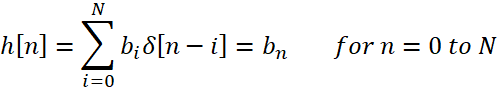
An FIR digital filter can be understood by considering the difference equation which defines how the input signal is related to the output signal as:
y[n] = b0x[n] + b1x[n-1] +...+bNx[n-N]
where x[n] is the current input signal sample, x[n-1] is the previous signal sample and x[n-N] is the last sample in the series. The series multiplies the most recent (N+1) samples associated with the (N+1) filter coefficients. y[n] is the current output signal and bi are the filter coefficients. The number N is known as the filter order; an Nth-order filter has (N+1) terms on the right-hand side and (N+1) filter coefficients also referred to as “taps”.
This equation illustrates why a higher order filter has a slower response time. It takes more samples and therefore more time for an event to work its way through the series until the output is no longer affected by the event as compared to a lower order filter with fewer coefficients.
The previous equation can also be expressed as a convolution of the filter coefficients and the input signal.

The impulse response of the filter shows how the historical data affects the current filtered value. The longer the impulse response, the farther the old data will affect the current filtered value. To find the impulse response we set:
x[n]=δ[n]
where δ[n] is the Kronecker delta impulse. The equation below shows that the impulse response for an FIR filter is simply the set of coefficients bn, as follows:
FIR filters are clearly stable, since the output is a sum of a finite number of finite multiples of the input values, which implies that it can be no greater than

times the largest value appearing in the input.
Data Windows in FIR Filters
In the academic world, hundreds of methods are available to design a FIR filter to meet various criteria. The Post Analyzer software includes the most popular filter design methods: Data Windows and Remez. Both methods are discussed below.
The Data Window FIR Filter Design method is the easiest to understand. The name "Window" comes from the fact that these filters are created by scaling a sinc (SIN(X)/X) function with a window such as a Hanning, Flat Top, etc. to produce the desired frequency effect.

A data window FIR filter is generated by starting with an ideal “brick-wall” shaped filter, which is a filter with vertical edges or zero transition band width as shown on the left. The brick-wall filter is specified by the cutoff frequencies and has band-pass amplitude of 1 and stop band amplitude of 0. The problem with the ideal brick-wall filter is that the time response oscillates forever and it requires an infinite number of filter coefficients. This ideal filter can be modified by applying a data window to force the time response to decay in a finite time. Of course, this degrades the shape of the ideal brick-wall filter performance. It introduces ripple, increases the transition band width, and decreases the stop band attenuation. However, it allows the filter to be defined by a finite number of filter coefficients. The filter performance can be modified by using different data windowing functions and making the tradeoff between filter order and response time. The user must choose these settings during the filter design. The parameters set during the filter design are: decimation, filter type (bandpass, low pass, etc.), filter order, window type, and cutoff frequencies.
The following figures show a comparison of different data window choices for the same filter settings. In all cases the low and high cutoff frequencies are 0.1 and 0.4 relative to the sampling frequency.


As shown in the pictures, different window methods produce different filter performance, i.e., different attenuation of the main lobe and side lobes. The best data window choice depends on the user’s specific application.
Remez Filters
The Remez Filter is a different method for designing a FIR filter. It is more computationally intensive than the data window method. A Remez filter is generated with iterative error-reducing algorithms designed to reduce the passband error. In addition to the parameters defined in the Data Window filter, Remez filters also allow the users to define the width of each transition band, the passband ripple, and the stop band attenuation.
The figure below shows an example of a filter design using the Remez method in the Post Analyzer software. The low and high cutoff frequencies are 0.1 and 0.4 relative to the sampling frequency. The number of filter taps is 67.

The software is intelligent enough to automatically calculate the total FIR filter length based on these criteria. For example, if the user asks for very high attenuation, very small ripple, or very sharp transition band, the filter length will be very high. The user must make tradeoffs between these parameters so that the appropriate filter length can be generated and used.
The graphs below show the results of an FIR filter applied to a swept sine signal. This signal was generated using the EDM VCS software, then imported into PA for post-processing. Then the signal was decimated using the DecimFilter operator, and subsequently passed through an FIR Remez bandstop filter with the settings pictured above. The result is a signal that is approximately equal to the original signal in the lowpass and highpass regions, near zero in the bandstop region, and has the expected transition band regions on either side of the bandstop region. The top graph shows the original signal, the middle graph shows the signal after being passed through the Remez filter, and the bottom graph shows the RMS of the filtered signal as a function of time.

IIR Real Time Digital Filters
Infinite impulse response (IIR) filters’ impulse responses decay very slowly but theoretically lasts forever. This is due to the fact that the filter input includes the measured signal as well as the filter output, creating a feedback path which results in the infinite impulse duration. In contrast, finite impulse response filters (FIR) have fixed-duration impulse responses.
The design procedures for IIR filters are somewhat more complicated than FIR filter design because there is no direct design method like the data window method for FIR filters. Instead, IIR filters are typically designed by starting with an ideal analog filter in terms of the frequency response characteristics such as the Chebyshev, Butterworth, or Elliptic filter. Then the analog filter is converted into a digital filter using a method known as the Bilinear transformation or impulse invariance method.
An IIR digital filter can be understood by considering the difference equation which defines how the input signal is related to the output signal as:
y[n] = b0x[n] + b1x[n - 1] + ⋯ + bpx[n - P] - a1y[n - 1] - … - aqy[n - Q]
where P is the feed-forward filter order, b_i are the feed-forward filter coefficients, Q is the feedback filter order, a_j are the feedback filter coefficients, x[n] is the input signal and y[n] is the output signal.
The previous equation can also be expressed as a convolution of the filter coefficients and the input signal:

which, when rearranged, becomes:

To find the transfer function of the filter, we first take the Z-transform of each side of the above equation, where we use the time-shift property to obtain:

We define the transfer function to be:

The transfer function gives the frequency response that relates the input to the output magnitude and phase.
In the Post Analyzer software, the user specifies the following parameters for an IIR filter: decimation, filter type, filter order, analog prototype, and cutoff frequencies.
Various analog filter types can be used as the basis for the IIR filter. The Butterworth Filter is the filter type that results in the flattest passband and contains a moderate group delay. Below are examples of Butterworth low-pass and band-pass filters.


The Chebyshev Type I Filter results in the sharpest passband cut off and leads to the largest group delay. The most notable feature of this filter is the significant ripple in the passband magnitude. A standard Chebyshev Type I Filter's passband attenuation is defined to be the same value as the passband ripple amplitude. Below are examples of Chebyshev Type I band-pass and high-pass filters.
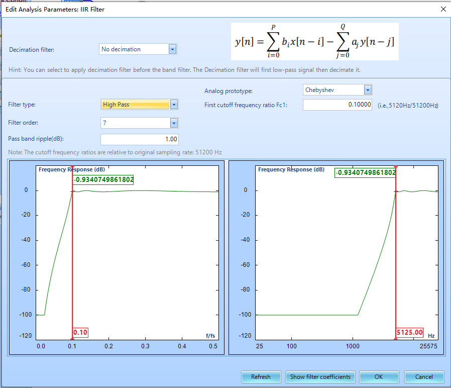

The Elliptic Filter contains a Chebyshev Type I-style equi-ripple passband, an equi-ripple stop band, a sharp cutoff, high group delay, and the greatest possible stop band attenuation. An equi-ripple frequency band is one in which all ripples have the same magnitude. Below are examples of 7th order Elliptic low-pass and band-stop filters.


The following is an example of an IIR filter applied to an input signal. The original signal was created by running a logarithmic swept sine test in EDM VCS from 10 to 2000 Hz. This signal was then imported into PA and processed using the steps shown below.

The incoming signal was first decimated so that it had a lower sampling rate. Then it was passed through a Butterworth style IIR filter with a bandpass from 50 to 512.5 Hz. Finally, the RMS of the output signal was calculated as a function of time. The results are shown in the graphs below. The top graph is the raw signal, the middle graph is the signal with the IIR filter applied, and the bottom graph is the RMS of the filtered signal as a function of time. One can see that the RMS starts out at approximately zero, but as the frequency of the sine wave enters the transition frequency range the RMS increases until it remains constant during the bandpass frequency range, and then drops off again during the second transition frequency range. This demonstrates clearly the effect of using an IIR bandpass filter.

Filters_RMS
This method involves calculating the RMS of the output of digital filters. While the results closely resemble the RMS output of 1/N octave filters, using Filters_RMS offers greater flexibility. Users can design any filter and examine its RMS output, providing a more versatile option.

Functionally, using the flow chart above does serve the same purpose. However, it is not convenient. The reality is that we mainly care about the final RMS value from one of the IIR band-pass filters. The intermediate results, such as the output time stream of the IIR filter, are not useful to us. Therefore, we can use Filter_RMS to directly calculate the data of interest, as shown below.

In addition to the IIR filters available for selection, Filter_RMS also allows you to select the other two FIR filters we introduced earlier in its Edit Parameters window, as shown below.

Applying Filters
In the PA software, filters can be applied to any project which supports the Data Conditioning option. Clicking on the Data Conditioning button in the toolbar at the top of the screen will bring up this module. Digital filters, as well as Math, Statistics, and other options can be found by clicking on the relevant tab at the bottom of the screen. The Edit Parameters button can be found in the Control Panel, which will bring up the edit window as shown below. Alternatively, users may double click the icon for the filter being used in the Data Conditioning window to configure the filter parameters as introduced in previous sections. Users may also right-click the filter icon to access a command to delete a module.

An example of the Data Conditioning module with different types of filters applied to a set of data is shown below.

Applying Digital Resampling
Digital resampling allows a user to convert a signal from one sampling rate to another after the signal has been collected. Similarly to Digital Filters, Resampling can be applied to any project supporting the Digital Resample option. This module can also be found under the Data Conditioning tab. There are two operations within the Resampling module: DecimFilter, which decreases the sampling rate, and Resampling, which increases the sampling frequency. DecimFilter applies a decimation filter to the input signal as described earlier. In the Control Panel, the user has the option to edit the decimation stage, which represents how many times the decimation filter is applied. Each application of the decimation filter reduces the sampling frequency by ½, therefore the final sampling frequency will be given by

where n is the decimation stage. The option to edit resampling rates can be found in the Control Panel.

Instead of adding the digital resample module at the Data Conditioning phase, the digital resample can also be set up in Project Configuration.