
An Ear for Gears - Understanding Gearbox Signatures
Speed reducers and other gearboxes are common industrial components. Monitoring their case vibration with accelerometers is an effective means of detecting problems within. To effectively diagnose these important mechanical elements, you need to understand the geometric details of their construction. Most importantly, you need to know the arrangement of shafts and the number of teeth on every gear within your transmission.
Consider the simplest system, two mating spur gears. Presuming the gearbox is a speed reducer, the input shaft has the smaller diameter of the two gears – we will call this the pinion. The pinion has Tp teeth on its perimeter, and these mate with the Tg teeth of the larger gear on the slower output shaft. The gear ratio (the speed reduction ratio), R, is defined as:

But knowing the number of teeth on the gear and pinion tell us much more than simply the speed reduction (torque multiplication) provided by the gearbox. Figure 1 illustrates the conventional numbering sequence of gear and pinion teeth as they enter mesh with one another. Now consider which gear teeth engage which pinion teeth during operation. We will look at three different sized gears mated to a 6-tooth pinion.
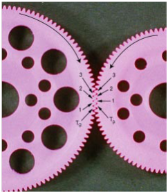
Figure 1: Tooth numbering convention
If the gear is of the same size (6 teeth), each pinion tooth only engages its numerically equal gear tooth as shown in figure 2. Thus pinion tooth #4 always transfers its load to gear tooth #4 (and no other) and so on. Since only like-numbered gear and pinion tooth-pairs are mated throughout their service life, it is likely they will develop complimentary wear patterns to compensate for any minute imperfections of manufacture. Should this gear pair be separated during a repair, the odds are 5 to 1 that this same arrangement of parts will not be restored unless the mating parts were marked at dis-assembly. In subsequent operation, the mating teeth will no longer have their hard-won complimentary wear patterns; this can cause a signature change.

Figure 2: Tooth mating sequence for 6-tooth pinion and 6-tooth gear
Now consider the entirely different situation illustrated by figure 3. Here, the same 6-tooth pinion drives a 7-tooth gear. Note that every pinion tooth eventually drives every gear tooth. All 42 mating combinations are encountered in seven pinion revolutions (6 gear revolutions). That is, this gear set can only be assembled in one way and there is no benefit to marking its parts at dis-assembly. Such a gear set is said to have one assembly phase in contrast to the gear set of figure 2 which has six assembly phases.

Figure 3: Tooth mating sequence for 6-tooth pinion and 7-tooth gear
Adding another tooth to our gear produces a situation between these extremes. As shown in figure 4, when a 6-tooth pinion drives an 8-tooth gear, every pinion tooth only comes into contact with four gear teeth and every gear tooth only engages three pinion teeth. By following the path lines between tooth-pair intersection points, you will note a given pair of teeth enters the mesh every 3 gear rotations (every 4 pinion rotations).

Figure 4: Tooth mating sequence for 6-tooth pinion and 8-tooth gear
We can summarize these observations by rewriting the gear ratio equation. Specifically:

Nap is the largest (integer) common factor between Tp and Tg. This common factor is the number of assembly phases possible between the pinion and gear, while tg is the number of gear teeth in the assembly phase and tp is the number of pinion teeth in the assembly phase.
Figure 5 makes these points graphically. It illustrates one of the 12 possible assembly phases between a 108-tooth pinion and a 120-tooth gear. In this case:

While all of the gear and pinion teeth participate in mesh, any tooth within this assembly phase can only contact the mate shown. Clearly, this gear pair may be assembled with twelve different tooth-mating sequences.

Figure 5: Mesh between 108-tooth pinion and 120-tooth gear exhibits 12 assembly phases; the teeth of one assembly phase are marked.
The frequencies defined by Equations (2) through (6) can all be expected to be present (with varying intensities) in any gearing signature. Invariably, f mesh will be a dominant component in any noise or vibration spectrum measured from a gearbox. Note that gear mesh is a much higher frequency than the shaft speeds, the assembly phase passage frequency and the “hunting tooth” frequency. In fact, all of these frequencies are integer sub-harmonics of f mesh. The hunting-tooth frequency is the lowest characteristic frequency of the gear-pair and the remaining characteristic frequencies are all integer harmonics of fhunting tooth.

where: RPMgear = the gear-shaft turning speed in RPM
and fgear = the (same) gear-turning frequency in Hertz

where: fpinion = the turning speed of the pinion shaft in Hertz

where: fmesh = the frequency at which teeth-pairs enter the gear mesh

where: fassembly pass = the frequency at which an assembly phase passes through mesh

where: fhunting tooth = the frequency at which a specific tooth-pair mates in mesh
Gears function to transmit torque from one shaft to another. In a perfect world, they would do so with the quiet smoothness of a pair of rolling elements in perfect contact with infinite friction at their juncture. Gear tooth profiles are carefully designed to pass load from one tooth to the next as smoothly as possible. They engage one another with an intended rolling contact and as little sliding as possible to preserve high efficiency. Unfortunately, perfection has eluded us and real gears perform this load hand-off between adjacent tooth-pairs with a certain amount of impacting, sliding, bending and other socially undesirable behavior. This “mating activity” repeats at the mesh frequency. Fmesh and its harmonics are always present in the noise and vibration spectra, most particularly when the gears are lightly loaded.
The remaining characteristic frequencies, fhunting tooth, fgear, fpinion and fassembly pass are normally less evident in a smooth gear-set. The shaft speeds fgear and fpinion may appear in vibration spectra due to unbalance of the driver or driven element. Second harmonics of these terms often accompany misalignment of shafting (or loose mounting of a drivetrain component). Generally, these frequencies indicate problems external to the gear-set.
In contrast, a small eccentricity of the pinion on its shaft will induce vibration at the sum and difference frequencies, fmesh + fpinion and fmesh - fpinion, while a similar problem with the gear will produce detectable activity at fmesh + fgear and fmesh - fgear. In general, the amplitude exhibited at a “sum frequency” will be (about) equal to that at the corresponding “difference frequency.” That is, the eccentricity signatures exhibit symmetric sidebands about the mesh frequency.
In practice, both the mesh frequency carrier and the (pinion or) gear-shaft frequency modulator can have many harmonics (of various phasing) present. This means that the resulting modulated signal can be more complicated with distinct tones appearing at frequencies of nfmesh ±kfgear, where n and k are integer constants. Normally, the terms symmetrically disposed about fmesh (where n equals 1) will dominate. Sidebands associated with low k value are usually the most detectable. Gear wear and clearance changes in plain bearings can cause a change in the fgear and fpinion sidebands. So can an unrelated repair that causes the gears to be re-mated with “new” assembly phasing. Such unintended signature change may also be accompanied by a rise in the ±fassembly pass sidebands of f mesh and its harmonics (when these terms are unique).
In a 1:1 gearing, Nap = Tp = Tg, so that tp = tg = 1. Hence, fassembly pass = fgear = fpinion and the assembly phase passage frequency is not a unique characteristic. When the gear-set is designed for uniform distribution of tooth wear, the gear and pinion tooth-counts share no prime numbers in common, save 1. In this circumstance, Nap = 1, resulting in fassembly pass = fmesh . Hence any ±fassembly pass sidebands of fmesh and its harmonics will appear as either an harmonic of fmesh or at DC; they will not be uniquely identifiable. In all other situations, fassembly pass is a unique characteristic frequency. Since fassembly pass is typically much higher than either fgear or fpinion, the ±fassembly pass sidebands of fmesh will be widely spaced from their carrier and are not likely to be confused as “high k” images of either fgear or fpinion.
Presence of the very low frequency fhunting tooth is a clear indicator of severe local tooth-pair damage such as that encountered when the mesh has “digested” a significant solid contaminant. This term also shows up as a pair of symmetric sidebands centered upon the mesh frequency. It is difficult to detect these fmesh ±fhunting tooth components and differentiate them from gear mesh (particularly in uniform tooth wear gearing) owing to the close frequency spacing. An order normalized analysis of at least TgTp/Nap lines of spectral resolution is required to detect these indicators. They are worth separating; when they are observed, they typically indicate local tooth damage that can be seen with the unaided eye.
If the gearbox you are diagnosing operated at a tightly regulated speed, all of these terms may be discernible in an ordinary FFT spectrum. However, if the machine speed varies (albeit slightly) with load, the resulting spectral peaks you wish to characterize will likely be blurred or smeared into the background across many frequency bins. The answer to this problem is to run the Order Tracking software on your handheld CoCo-80/90 or modular Spider-80X front end. This optional software phase-locks the sample rate of your analyzer to the speed of a shaft by synchronizing on a pulse tachometer signal. Digital re-sampling of the data provides a matching speed-tracking anti-aliasing filter.
Figure 6: Block diagram of the Order Tracking measurement process
In fixed-bandwidth operation, an analyzer collects N successive samples from an analog time-history at a constant sample rate, fs. The analog signal is pre-filtered by a low-pass anti-aliasing filter set to the desired analysis frequency range, Fspan and the sample rate is set to k Fspan, where k is a constant specific to the analyzer. Each captured time-history is transformed to yield a spectrum. The following spans and resolutions result:
Δt = 1/fs = 1 / k Fspan time between adjacent time points (S)
Tspan = N Δt duration of each time capture or memory load period (S)
ΔF = 1/Tspan difference between adjacent frequency points (Hz)
Fspan = N ΔF / k frequency range presented (Hz)
In order-normalized (order-tracked) analysis, both the frequency range and sample rate must vary in proportion to the machine speed. This is accomplished by measuring the shaft speed with a tachometer and deriving a sample rate equal to k Ospan times the instantaneous shaft speed. Ospan is the maximum number of shaft-speed orders (multiples) to be measured in a spectrum. The effective anti-aliasing filter must constantly adjust to limit the incoming signal bandwidth to Ospan times the shaft-turning frequency. This results in the following spans and resolutions:
ΔR = 1/fs = 1 / k Ospan shaft-angle between adjacent signal samples (Revolution)
Rspan = N ΔR number of turns in each memory capture (Revolution)
ΔO = 1/Rspan difference between adjacent order points (Order)
Ospan = N ΔO / k order span presented (Order)
Typical analyzers require between 2.56 and 4 samples per maximum order spanned. This is the same k multiple relating the analyzer’s sample-rate to the frequency band studied in normal fixed-bandwidth analysis. The exact numeric value is determined by the analyzer’s design specifics.