
Modal Analysis of Airplane Model Using EDM Modal
Analyzing the modal parameters of a structure is crucial in optimizing the mechanical properties of the test object. The natural frequencies, damping and mode shapes of the unit under test help in adjusting the design of the test structure which ultimately improves the structural behavior of the test unit. Hence, modal analysis is a vital process of product development.
In this case, the modal characteristics of an airplane model is acquired by performing experimental modal analysis. A SIMO FRF test is carried out using a single modal shaker and multiple sensors to obtain the vibration characteristics. Shaker excitation provides better consistency and repeatability than a modal hammer. It also produces a cleaner data set because of a greater average. The higher quality measurements lead to a better estimation of the modal parameters.
To avoid the mass loading effect that is induced with a roving response measurement, the entire modal test is carried out in a single run. A total of 25 sensors are attached on all the corresponding measurement points to capture the response of the entire plane in one shot.
The high-channel count Spider-80Xi system aids in executing this test. The latest 8.1 release of the EDM Modal software assists in executing the SIMO FRF test.

Figure 1. Modal shaker testing of the airplane model
A mesh configuration of 25 measurement points is placed over the front and rear wings. Using flexible bands and bungee cords the plane is suspended to imitate a free-free boundary condition (as shown in the experimental setup). The modal shaker is attached to the center of the plane to excite the global modes. The responses to the shaker excitations are captured using 24 uni-axial accelerometers and 1 impedance head that are uniformly distributed throughout the wings. Measuring the excitation and response in the vertical direction facilitates in obtaining the out-of-plane mode shapes.

Figure 2. Airplane geometry
For this modal test, the lower order modes are of interest and therefore a sampling rate of 1 kHz is set. A block size of 2048 is selected. A fine frequency resolution of 0.488 Hz is produced with these configuration settings. Measurements of higher accuracy and reduced noise are obtained by linearly averaging 28 blocks of data at each measurement DOF.
Burst random excitation imparts energy across a broad frequency range of 450 Hz and has the added advantage of user tunable burst percentage to control the no output duration time which allows the responses to decay to zero. With this setup, there will be no leakage and the uniform window can be selected. For this test, the output amplitude was set to 0.2 V with an 80% burst rate.

Figure 3. SIMO FRF measurement of the airplane
The 80% burst rate ensures that the shaker provides excitation for 1.64 seconds in each time block and there is no output for the remaining 0.41 seconds. This information is graphically represented in the plots shown above.
The coherence plot is acceptable. The valleys in the coherence plot occur at the anti-resonances which indicates that the response level is relatively lower at these corresponding frequencies. So overall, the inputs and outputs are well correlated in the desirable frequency range.
The FRF measurement shows good dominant peaks in the 0-150 Hz frequency band. Plotting the imaginary part of all the FRFs guides allows users to observe the phase relationship between the measurement DOFs. The well aligned peaks on the imaginary portion of the FRFs indicates that there is no mass loading effect induced in the results.

Figure 4. Modal Data Selection tab showing the imaginary part of all overlapped FRFs
The new Poly-X method is used to curve-fit the FRF’s in 2 stages to procure the following stability diagrams. Five flexible modes and one rigid body mode are selected within the desired frequency range. The Multivariate Mode Indicator Function (MMIF) is used to indicate the valleys at the natural frequencies.

Figure 5. Stability diagram for the first frequency band

Figure 6. Stability diagram for the second frequency band
The Auto-MAC matrix helps in validating the results. The Auto-MAC matrix below shows that the modes are orthogonal to each other (low off-diagonal elements) and are uniquely identified (high diagonal elements).

Figure 7. Auto MAC chart for the airplane SIMO modal test
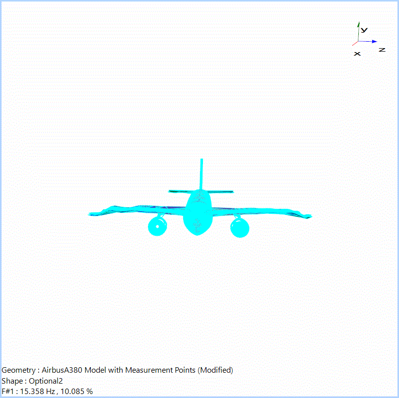
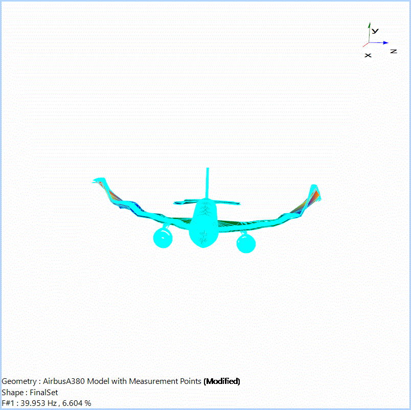
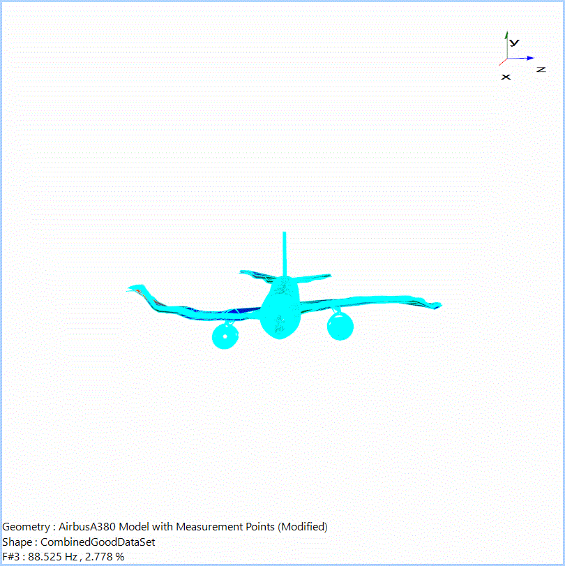
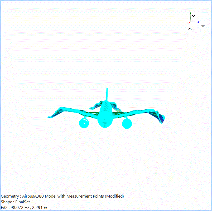
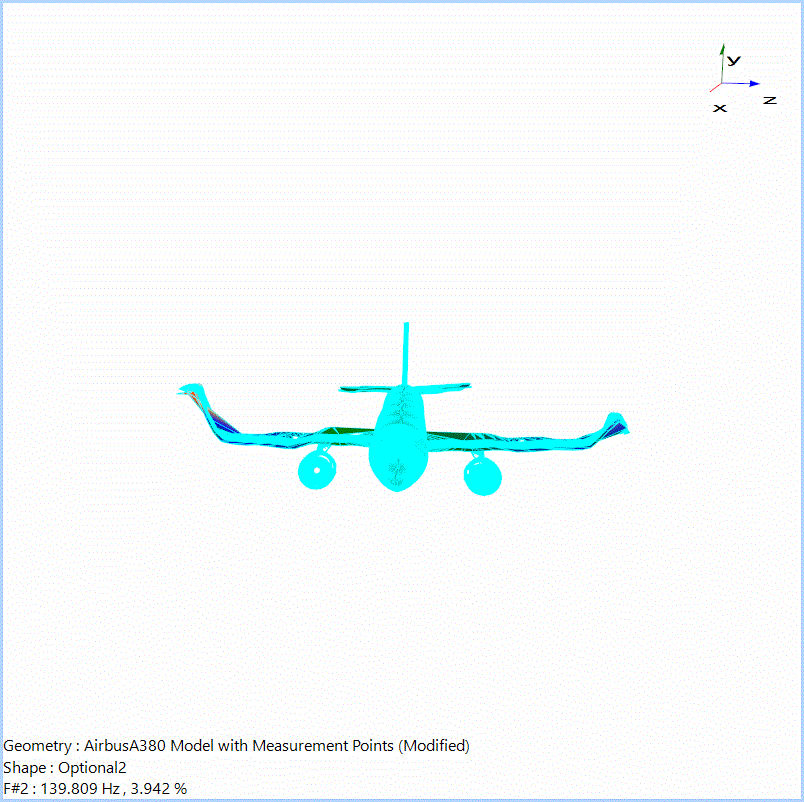
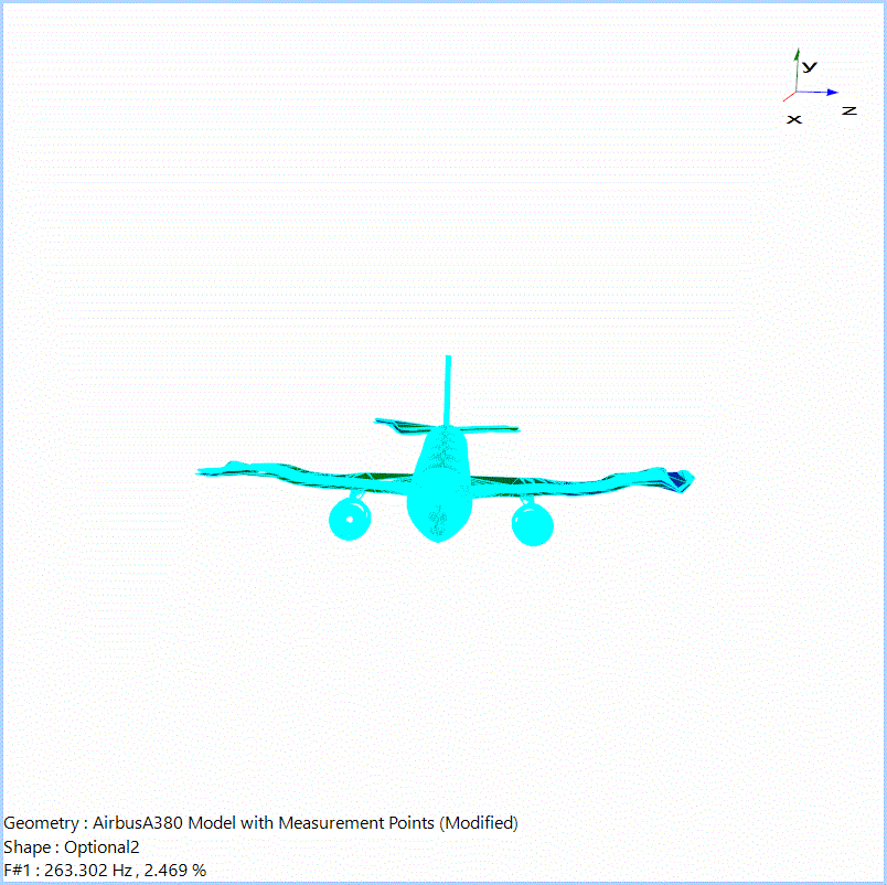
The animation shapes of the rigid body mode and the flexible body modes associated with the stable physical poles are shown below.
The results display the strength of the high-channel count Spider-80Xi system and the efficiency of the EDM Modal software to execute sophisticated modal tests on complex structures.
To learn more about EDM Modal software, visit: www.crystalinstruments.com/edm-modal-testing-and-analysis-software/